Fatou and Julia

Complex dynamics is the study of iterations of a holomorphic map $f: X \to X$ where $X$ is a Riemann surface. Dynamical objects of interest are the Fatou set $F(f)$, i.e. the subset of $X$ on which the iterations are stable, and the Julia set, which is the unstable region. Below, I am to summarise the basic concepts of Fatou and Julia sets in one-dimensional complex dynamics. I will focus on the case where $X$ is an open subset of the Riemann sphere $\mathbb{P}^1 = \mathbb{C} \cup {\infty}$. Proofs will be skipped and I would personally recommend referring to Beardon¹ or Milnor² for more details.

A collection $\mathcal{F}$ of continuous functions from topological spaces $A$ to $B$ is called a normal family if it is precompact with respect to the compact-open topology. That is, every sequence of functions $f_n$ in $\mathcal{F}$ contains a subsequence which converges uniformly on compact subsets of $A$ to a continuous function $f: A \to B$, not necessarily in the family $\mathcal{F}$. A simple example would be the family of linear maps $\mathcal{F} = \{ \mathbb{P}^1 \to \mathbb{P}^1, z \mapsto 2^{-n} z \}_{n \in \mathbb{Z}}$. It is is normal because any infinite sequence of maps in $\mathcal{F}$ subsequentially converges to either a map in $\mathcal{F}$, the zero map $z \mapsto 0$, or the infinity map $z \mapsto \infty$.

When $A \subset \mathbb{P}^1$ and $B = \mathbb{P}^1$, Arzelà–Ascoli theorem implies that normality is equivalent to equicontinuity of $\mathcal{F}$ with respect to the spherical metric $d$ on $\mathbb{P}^1$. When the family $\mathcal{F}$ is the set of iterates $\{f^n\}_{n \in \mathbb{N}}$ of a holomorphic function $f: A \to \mathbb{P}^1$, equicontinuity means that for all $\epsilon >0$, whenever two points $z$ and $w$ are sufficiently close, then for any iterate $f^n$, $d(f^n(z),f^n(w)) < \epsilon$. This is our notion of stability.

We then define the Fatou set $F(f)$ of a holomorphic map $f: X \to X$ as the open set of points $z \in X$ such that there is a neighbourhood of z on which $\{f^n\}_{n \in \mathbb{N}}$ is a normal family. The Julia set of $f$ is the closed set $J(f) = \mathbb{P}^1 \backslash F(f)$. Checking the normality assumption can be rather tedious. A commonly used tool is the following result by Montel.

Montel’s Theorem: If $\mathcal{F}$ is a family of holomorphic maps from a hyperbolic Riemann surface $A$ to $\mathbb{P}^1 \backslash K$ for some compact subset $K$ containing at least 3 distinct points, then $\mathcal{F}$ is a normal family.

Here, hyperbolic means that the universal cover of $A$ can be taken to be the unit disk $\mathbb{D}$. The good news is that, by uniformisation theorem, most Riemann surfaces are hyperbolic. Every non-hyperbolic surface is either $\mathbb{P}^1$, $\mathbb{C}$, the punctured plane $\mathbb{C}^*$, or a complex torus. (In particular, $\mathbb{P}^1 \backslash K$ is hyperbolic.) Montel’s theorem immediately guarantees that the Julia set of $f$ is empty when $\mathbb{P}^1 \backslash X$ contains at least three distinct points. When $X$ is a complex torus, Milnor² $\S 6$ explained clearly that $J(f)$ is either empty or $X$. This leaves $X$ being either $\mathbb{P}^1$, $\mathbb{C}$ or $\mathbb{C}^*$ as the only non-trivial cases.

Let’s look some easy examples when $X=\mathbb{P}^1$.

• If $f$ is a rotation $f(z) = e^{i\theta} z$, $F(f) = \mathbb{P}^1$ because $f$ is an isometry with respect to the spherical metric and the family of iterates is automatically equicontinuous.
• If $f(z) = az$ for some $a \in \mathbb{C}$ where $\lvert a \rvert < 1$, $F(f) = \mathbb{C}$ since we can apply Montel’s theorem to any finite disk centered at $0$, but on any neighbourhood $N$ of $\infty$, $\mathbb{C} \subset \cup_{n=1}^\infty f^n(N)$.
• Similarly, if $f(z) = z+a$ is a translation, $F(f) = \mathbb{C}$ and $J(f) = \{ \infty \}$.
• By classification of Möbius transformations on $\mathbb{P}^1$, the Julia set of any Möbius transformation is either empty or a singleton.
• If $f(z) = az^n$ where $\lvert a \rvert = 1$ and $n \geq 1$, $J(f)$ is the unit circle.

Below are some dynamical properties of the Julia set (and consequently the Fatou set as well).

Proposition: Let $f: X \to X$ be a holomorphic map on an open subset $X \subset \mathbb{P}^1$.

1. The Julia set of $f$ is completely invariant: $f^{-1}J(f) = J(f) = f J(f)$.
2. For any $n \in \mathbb{N}$, $J(f^n) = J(f)$.

Recall that a point $z_0 \in X$ is a periodic point of (prime) period $n$ if $n$ is the smallest positive integer such that $z_0$ is a fixed point of $f^n$. Its multiplier $\lambda$ is the derivative $(f^n)’(z_0)$. (When $z_0 = \infty$, pass it to the chart $z \mapsto z^{-1}$ about $\infty$.) We say that $z_0$ is attracting if $\lvert \lambda \rvert<1$, repelling if $\lvert \lambda \rvert>1$, and indifferent if $\lvert \lambda \rvert=1$.

The different types of a periodic point $z_0$ tell us the behaviour of iterates near $z_0$. For every point $w$ in a small neighbourhood $U$ of $z_0$, $f^n(w) \to z_0$ if attracting, and there is some $n$ where $f^n(w)$ escapes $U$ if repelling. The behaviour when $z_0$ is indifferent is almost always a saddle or rotational, though it can be much more complicated. (This nonsense is called the Cremer periodic point.)

Using the vocabulary above, another useful way of characterising the Julia set is the following.

Theorem: The Julia set $J(f)$ is the closure of the set of all repelling periodic points of $f$.

Computing the Julia set by finding each repelling periodic point is computationally intensive and, in fact, almost impossible. Instead, one possible approach is to find one repelling periodic point, we can find its iterated preimages. This is made possible by the following result.

Proposition: If $z_0 \in J(f)$, then the closure of the set of preimages $\bigcup_{n=1}^\infty f^{-n}\{z_0\}$ of $z_0$ is the Julia set.

The method of iterated preimages works best when the map $f$ has a small finite degree and is somewhat ‘nice’ enough. When it has high or infinite degree, finding the Julia set may still be computationally heavy. The gifs below provide two examples of how the preimages of the repelling fixed point of $z^2 + 0.25$ and $z^2-0.8+0.25i$ respectively approximate the Julia set.

We will offer another approach using attracting periodic points. Denote by $\mathcal{A}(z_0)$ the basin of attraction of the orbit of an attracting periodic point $z_0$. Using the spherical metric $d$, this set can be defined as

When we are blessed with the presence of an attracting periodic point $z_0$, we can obtain the Julia set for granted.

Proposition: If $z_0$ is an attracting periodic point of $f$, then the boundary of its attracting basin $\mathcal{A}(z_0)$ is the Julia set $J(f)$.

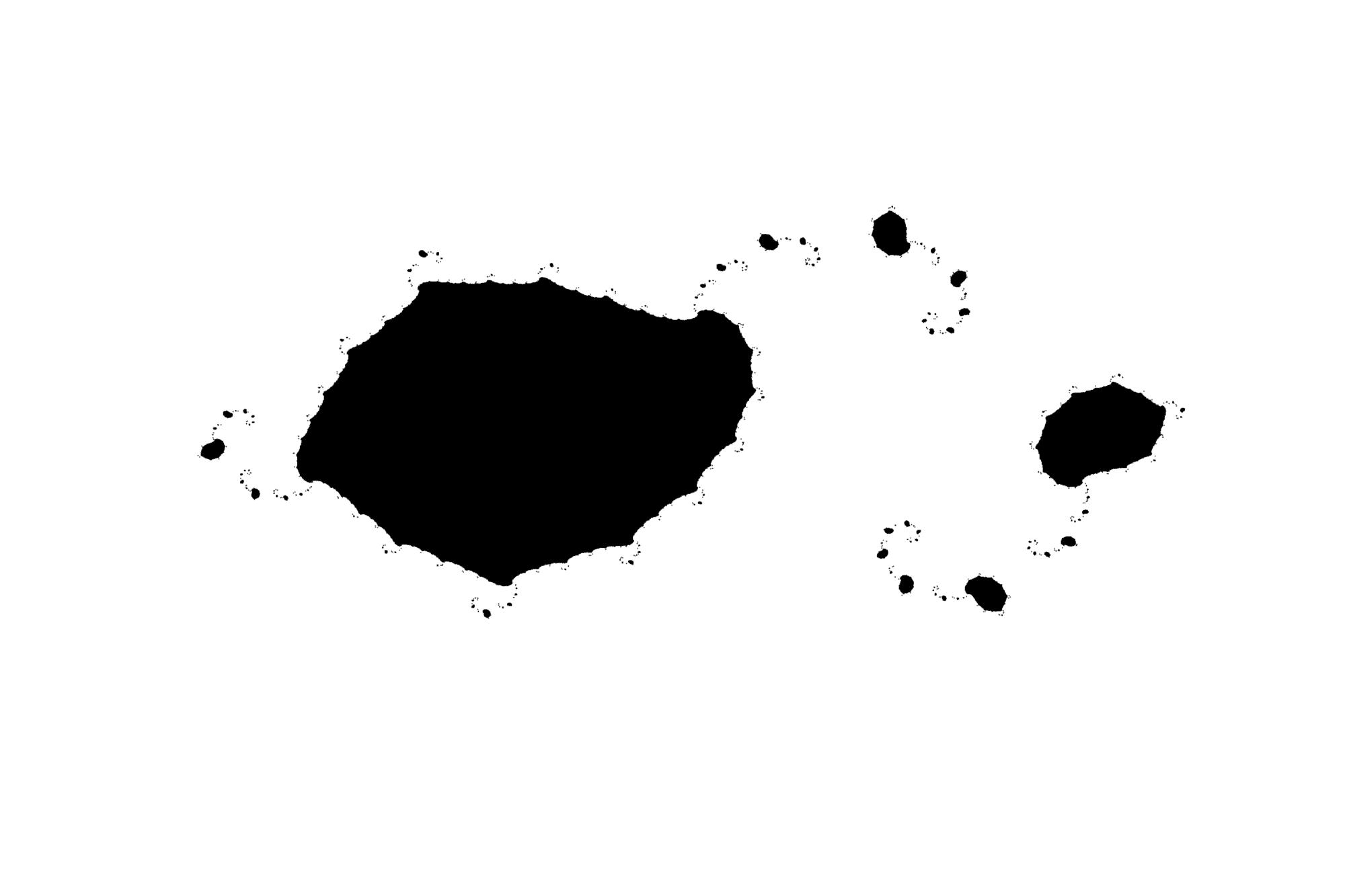
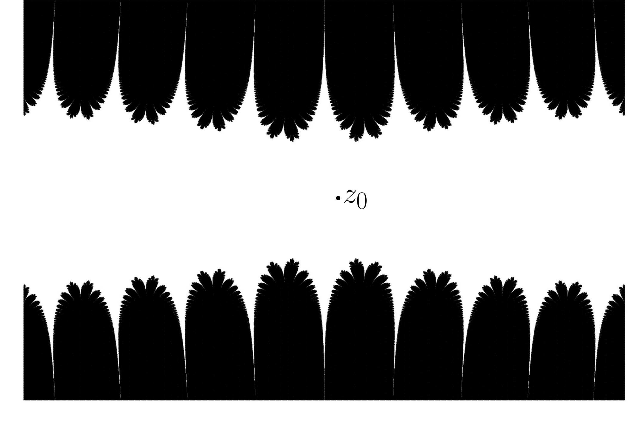
One special case is when $f$ is a polynomial of degree $d \geq 2$. This map always has a (super)attracting fixed point at $\infty$, and upon finding which points iterate away towards $\infty$, we obtain the attracting basin of infinity $\mathcal{A}(\infty)$ and its boundary is the Julia set $J(f)$. The complement $K(f) := \mathbb{P}^1 \backslash \mathcal{A}(\infty)$ is often called the filled Julia set. Below are the filled Julia set of $(-0.4+0.1i)(z^3-3z-2)-1$ and the complement of the attracting basin of the fixed point $z_0 = 0.8767\ldots$ of the transcendental map $\frac{\sin z}{z}$.

References

1: A. Beardon. Iteration of Rational Functions. Grad. Texts Math. 132, Springer-Verlag, NY, 1984.
2: J. Milnor. Dynamics in one complex variable. Princeton University Press, third edition, 2006.