Extremal length

Extremal length measures the size of curve families in a way that is invariant under conformal mappings. The extremal length also gives a way to define quasiconformal maps, i.e. orientation preserving homoeomorphisms which distort angles locally up to some bounded constant, and equivalently, distort extremal lengths up to some bounded constant. In this post, I aim to discuss the basic concepts of extremal length.

Consider a non-empty open subset $D \subset \mathbb{C}$ of the complex plane and the set $W_D$ of all measurable functions $\rho : D \to [0,\infty)$ such that $D$ always has finite positive $\rho$-area $A_\rho (D) = \int_D \rho^2 dx dy$. The extremal length $\lambda(\Gamma)$ of a collection of rectifiable curves $\Gamma$ in $D$ is defined to be

where $L_{\rho} (\Gamma)$ is the infimum of $\rho$-lengths $L_\rho (\gamma) = \int_\gamma \rho \vert dz\vert$ of curves $\gamma \in \Gamma$.

Some Properties

Extremal length gives us a measurement of curve families that is invariant under conformal maps. For this reason, its study has a variety of uses in complex analysis.

Proposition: Let $f: U \to V$ be a biholomorphism of two domains $U, V$ in $\mathbb{C}$. For any family of rectifiable curves $\Gamma$ on $U$, if $f(\Gamma) = \{ f\circ \gamma \}_{\gamma \in \Gamma }$, then $\lambda( f(\Gamma) ) = \lambda( \Gamma)$.

The intuition behind the proof is fairly simple. Due to conformality of $f$, we have a bijection of weight functions $f^* : W_V \to W_U, \rho \mapsto f^* \rho$ where the pullback is defined by $f^*\rho(z) = \rho(f(z)) \vert f’(z)\vert$ for all $z \in U$. By the change of variables formula, $A_\rho (V) = A_{f^*\rho} (U)$ and $L_\rho( f(\gamma)) = L_{f^*\rho} (\gamma)$ for every $\gamma \in \Gamma$.

Proposition Suppose that $\Gamma_1$ and $\Gamma_2$ are curve families in a domain $U$ such that each curve in $\Gamma_1$ is disjoint from curves in $\Gamma_2$, and vice versa. Denote by $\Gamma_1 * \Gamma_2$ as the family of concatenated curves $\gamma_1 * \gamma_2$. Then, we have the following laws.
(1) Parallel law: $\lambda(\Gamma_1 \cup \Gamma_2)^{-1} \geq \lambda(\Gamma_1)^{-1} + \lambda(\Gamma_2)^{-1}$;
(2) Series Law: $\lambda(\Gamma_1 * \Gamma_2) \geq \lambda(\Gamma_1) + \lambda(\Gamma_2)$.

The majority of the proof relies on direct $\sup$ and $\inf$ arguments. I’d recommend looking at Ahlfors¹ for more details.

Some examples

To get the idea of what extremal length is and how it can be computed, let’s look at some easy examples.

Let’s have a look at the regular rectangle $R = \{ x+iy : \vert : 0\leq x \leq a, 0 \leq y \leq b \}$ of side lengths $a>0$ and $b > 0$ and the family $\Gamma$ of rectifiable curves in $R$ joining the left vertical side with the right vertical side. Pick any arbitrary $\rho \in W_R$. Horizontal curves $\gamma_y(x) = x+iy$, $0 \leq x\leq a$, for fixed values of $y \in [0,b]$ belong in $\Gamma$. Since $L_{\rho} (\Gamma) \leq L_\rho (\gamma_y)$,

By Cauchy-Schwarz,

Upon rearrangement, we obtain an upper bound: $\lambda(\Gamma) \leq \frac{a}{b}$. The upper bound is indeed achieved by the Euclidean weight $\rho \equiv 1$ because in this case, $A_\rho(R)$ is the usual area $ab$ of the rectangle and $L_\rho (\Gamma)$ is the minimal length $a$ of curves in $\Gamma$. Therefore, the extremal length of $\Gamma$ is $\frac{a}{b}$. This quantity is more commonly known as the modulus $\text{mod}(R)$ of the rectangle $R$.

Let’s look at another example. Consider the family $\Gamma$ of rectifiable curves in the concentric annulus $\mathbb{A}_{r_1,r_2} = \{ r_1 \leq \vert z\vert \leq r_2 \}$, where $0<r_1<r_2<\infty$, which join the two boundary components of $\mathbb{A}_{r_1,r_2}$. Pick any arbitrary $\rho \in W_{\mathbb{A}_{r_1,r_2}}$. Radial curves $\gamma_\theta(r) = re^{i\theta}$, $r_1 \leq r \leq r_2$ for fixed angles $\gamma \in [0,2\pi)$ belong in $\Gamma$. Since $L_{\rho} (\Gamma) \leq L_\rho (\gamma_\theta)$,

By Cauchy-Schwarz,

Upon rearrangement, we obtain an upper bound $\lambda(\Gamma) \leq \frac{1}{2\pi} \log\left(\frac{r_2}{r_1}\right)$. This upper bound is again achieved by the weight function $\rho(re^{i\theta}) = \frac{1}{r}$, so the extremal length of $\Gamma$ is indeed $\frac{1}{2\pi} \log\left(\frac{r_2}{r_1}\right)$. This quantity is again called the modulus $\text{mod}(\mathbb{A}_{r_1,r_2})$ of the regular annulus $\mathbb{A}_{r_1,r_2}$. In the case where $r_1 = 0$ and/or $r_2 = \infty$, we set the modulus to be $\infty$. Observe that we can also obtain the modulus from the conformal map $R \to \mathbb{A}_{r_1,r_2}, z \mapsto r_1 e^{2\pi z/b}$ where the sides $a$ and $b$ of the rectangle $R$ are picked such that $\frac{r_2}{r_1} = e^{2\pi a/b}$. This conformal map should give you a hint on the equivalence between $\text{mod}(R)$ and $\text{mod}(\mathbb{A}_{r_1,r_2})$.

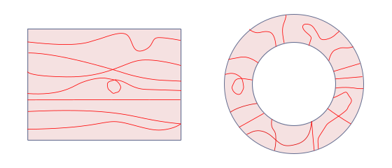
By conformal invariance, we see that the modulus of a regular rectangle is a conformal invariant. We can define the modulus of a topological annulus $\Omega$ either as the extremal length of the family of rectifiable curves in $\Omega$ joining the two boundary components, or as the modulus of a concentric annulus $\Omega’$ biholomorphic to $\Omega$. We can also define similarly the modulus of an arbitrary topological quadrilateral $Q = (Q,a_1,a_2,a_3,a_4)$, which is a Jordan disk in $\mathbb{C}$ equipped with four vertices $a_i$ for $i=1,2,3,4$ lying on the boundary $\partial Q$ and labelled cyclically in a counterclockwise manner. We additionally require that the biholomorphism sends vertices to vertices accordingly.

Weyl’s Lemma

We say that an orientation preserving homeomorphism $f: U \to V$ between domains $U,V$ in $\mathbb{C}$ is $K$-quasiconformal if there is some $K \geq 1$ such that every family of rectifiable curves $\Gamma$ in $U$ satisfies the following inequality:

In other words, these maps distort extremal lengths up to some bounded factor. It may not be obvious but this definition is in fact equivalent with the other definitions I have introduced in my previous post. Quasiconformal maps naturally generalise conformal maps because of the following result.

Weyl’s Lemma For an orientation preserving homeomorphism $f: U \to V$, the following are equivalent:
(1) $f$ is conformal;
(2) $f$ preserves extremal lengths;
(3) $f$ is 1-quasiconformal.

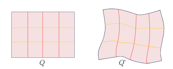
The only non-obvious implication is (3) $\Rightarrow$ (1). This is automatically true if $f$ is $C^1$, but in general we have to be more careful. We will follow directly from Ahlfors’ approach¹ using parallel and series laws. Suppose $f$ is $1$-quasiconformal and pick any arbitrary regular rectangle $Q \subset U$ of some modulus $m>0$. Draw some arbitrary disjoint vertical line segments to partition $Q$ into $Q_1, Q_2, \ldots Q_k$ for some $k\in \mathbb{N}$. Let $m_i$ be the modulus of each $Q_i$, then clearly $m = \sum_i m_i$. Denote by $Q’$ and $Q’_i$ the images of $Q$ and $Q_i$ for $i = 1, 2,\ldots k$ under $f$. By the assumption, $Q’$ and $Q’_i$’s have moduli $m$ and $m_i$.

By drawing some $l-1$ disjoint curves in $Q’$ joining the vertical sides, partition each $Q’_i$ into $Q’_{i1}, Q’_{i2}, \ldots Q’_{il}$ in such a way that $m_i^{-1} = \sum_j m_{ij}^{-1}$, where $m_{ij}$ denotes the modulus of $Q’_{ij}$. We first claim that the corresponding dividing horizontal curves in $Q$ must be straight line segments. There is a unique conformal map $g : Q’ \to Q$ preserving the vertices. Since the moduli matches, $g$ sends each $Q’_i$ to $Q_i$ and $Q’_{ij}$ to $Q_{ij}$. As the subdivision is arbitrary, $g$ must be the inverse of $f$. Therefore, $f$ is conformal on $Q$. As $Q$ is an arbitrary rectangle in $U$, $f$ is conformal on $U$.

What remains is to show that the claim holds. This subproblem can be simplified as follows. Let $l$ be a vertical curve dividing the rectangle $R = \{ x+iy : \vert : 0\leq x \leq m, 0\leq y \leq 1 \}$ of modulus $m$ into two open quadrilaterals $R_1$ and $R_2$ of moduli $m’$ and $m’’$. We need to show that if $m’ + m’’ = m$, then $l$ is the vertical line segment $\{x=m’\}$. Indeed, we can find two conformal maps

and let $\rho(z) = \vert f_i’(z)\vert$ if $z \in R_i$ for $i=1,2$, and $0$ if otherwise. Then,

and by Cauchy-Schwarz

Therefore, $\iint_R (\rho-1)^2 dx dy = \iint (\rho^2 - 1) - 2(\rho -1) dx dy \leq 0$, which immediately implies that $\rho$ must be $1$ almost everywhere in $R$. As such, $f_i$’s must be identity maps and $l$ must be the vertical line $\{x=m’\}$. All in all, the claim holds and (3) does imply (1).

Next time, I aim to post more about what makes quasiconformal maps interesting and what we can do with them.

References

1: L. Ahlfors. Lectures on Quasiconformal Mappings. Van Nostrand, 1966.