Iterated function systems

In simple terms, an iterated function system (IFS) is a set of contractions of a metric space. Each IFS admits a unique set invariant under iterations of these contractions, called the attractor of the IFS. IFS provides a robust method of generating fractals, and conversely the Collage Theorem states that any set can always be approxiated by the attractor of some IFS. In this post, I will describe the elementary theory of IFS and how it works.

Contractions

Let $(X,d)$ be a complete metric space and let $Y \subset X$ be a non-empty closed subset. A function $f:Y \to Y$ is a contraction if there is some ratio $r<1$ such that $d(f(a),f(b)) \leq r\cdot d(a,b)$ for all $a,b \in Y$. It is a straightforward exercise to show that contractions are always continuous. Also, global contractions are always dynamically simple as they are governed by one of the most popular fixed-point theorems out there.

Banach Fixed-Point Theorem: Given any contraction $f:X \to X$, $f$ has a unique fixed point $z$ and for any $x \in X$, $f^n(x) \to z$.

The proof is an elementary exercise in analysis: you can show that given any starting point $x$, the forward orbit $f^n(x)$ is a Cauchy sequence and therefore converges to a limit, which turns out to be the unique fixed point of $f$.

An iterated function system is a finite collection of contractions $\{ f_i: Y \to Y \}_{i=1,\ldots N}$. A non-empty compact subset $Z \subset Y$ is called an attractor of the IFS ${f_i}$ if $Z = \cup_{i=1}^N f_i(Z)$.

Let $\mathcal{C}$ denote the set of all non-empty compact subsets of $Y$. The metric $d$ induces the Hausdorff metric $D$ on $\mathcal{C}$ defined by

where $A_\epsilon$ is the closed $\epsilon$-neighborhood of $A$ (and similarly $B_\epsilon$). It is known that when $(X,d)$ is a complete metric space, $(\mathcal{C},D)$ is also a complete metric space.

The Hutchinson operator $F: \mathcal{C} \to \mathcal{C}$ defined by $F(A) = \cup_{i=1}^N f_i(A)$ is a contraction with respect to the Hausdorff metric because for any $A,B \in \mathcal{C}$,

Attractors of ${f_i}$ are simply fixed points of the Hutchinson operator. Therefore, we can adapt the Banach fixed-point theorem and obtain:

Hutchinson’s Theorem: Every IFS $\{ f_i: Y\to X \}_{i=1,\ldots N}$ on a closed set $Y \subset X$ admits a unique attractor $Z$. Moreover, for any $A \in \mathcal{C}$, $F^n(A) \to Z$ in $\mathcal{C}$.

Not only does this tell us that the attractor is unique, but it also tells us how to get the attractor as the limit of $F^n(A)$ for any non-empty compact subset $A$. Yes, $A$ can be picked to be either the whole $Y$ or even a singleton in $Y$, and it still works!

The Collage theorem

Given an IFS, we know how to obtain the corresponding attractor. What about the converse? If I pick my favorite compact fractal set, can I find an IFS whose attractor is close to my chosen set? The answer is yes!

The Collage Theorem: Given any non-empty compact subset $A$ of $Y$ and any IFS $\{f_i\}_{i=1,\ldots N}$ on $Y$ with attractor $Z$ and maximum contraction factor of $0<r<1$, we have

The proof of the theorem is fairly simple. Let $F$ be the corresponding Hutchinson operator. Then, the Hausdorff distance between $A$ and $Z$ has to be at most the value of the convergent series $D(A, F(A)) + D(F(A),F^2(A)) + D(F^2(A),F^3(A)) + \ldots$. Since $F$ is a contraction of factor $r$, each term in the series satisfies $D(F^i(A), F^{i+1}(A)) \leq r^i D(A,F(A))$ and we are left with an infinite series which becomes the right hand side of our inequality.

How is this useful? Given a compact set $A$, we can search for an IFS ${f_i}$ such that the collage of the images $f_i(A)$ is approximately close to $A$. Then, the theorem says that the attractor of the IFS should also be close to $A$. When the set $A$ that we start with is wild and computationally difficult to render, you can instead encode it with a good approximating IFS and render its attractor. This can be computationally handy when our contractions are simple (e.g. affine). However, the downside is that the number of contractions you need to consider may be arbitrarily large, especially if the set $A$ is wild and if you only allow very small error.

Some examples

The standard example you will find in almost all textbooks in fractal geometry is the middle third Cantor set. The generating IFS can be picked to consist of two contractions $f_1(x) = \frac{x}{3}$ and $f_2(x) = \frac{x+2}{3}$ of the unit interval $[0,1]$.

Here’s a cool way to draw a tree out of an IFS. We pick the IFS $\{f_i\}_{i=1,\ldots 6}$ consisting of six affine contractions $f_i$ of the plane that map the square $[-0.5,0.5]\times [0,1]$ to each of the following six parallelograms below. The gray ones correspond to $\{f_i\}_{i=3,4,5,6}$.

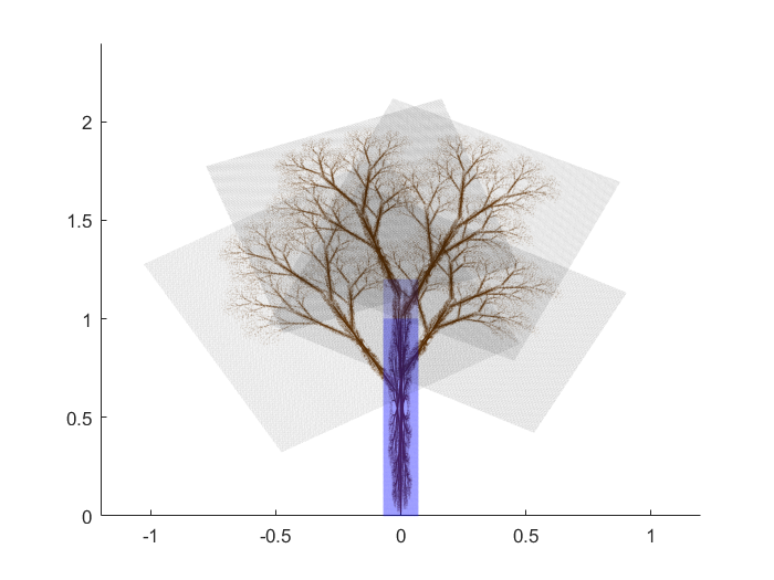
Let’s plant a square seed $S=[-0.1,0.1] \times [0, 0.2]$. Here’s a gif illustrating the first twelve iterates of $S$ under the Hutchinson operators corresponding to $\{f_i \}_{1\leq i \leq 6}$ (in brown) and $\{f_i\}_{3\leq i \leq 6}$ (in green). What do you see? :)

References

1: M. Barnsley. Fractals Everywhere. Academic Press, 1993.
2: K. Falconer. Fractal Geometry: Mathematical Foundations and Applications. John Wiley and Sons, third edition, 2014. ——